Correction du TD n°1 : Parmétrage - MGI, MGD d’un robot SCARA

On étudie le robot Scara 4 axes, référencé « s600 » de marque Adept.

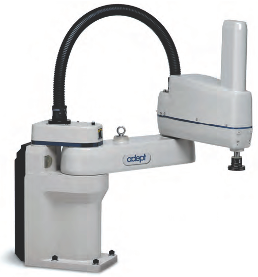
Fig. 28 Robot SCARA s600

Paramétrage

Question 1.1 : En se basant sur la documentation technique fournie en Annexes, proposer un schéma cinématique de ce robot.

Solution

Question 1.2 : Construire sur le schéma, la paramétrisation au sens de Denavit et Hartenberg modifée. Synthétiser les résultats dans le tableau associé.

Solution

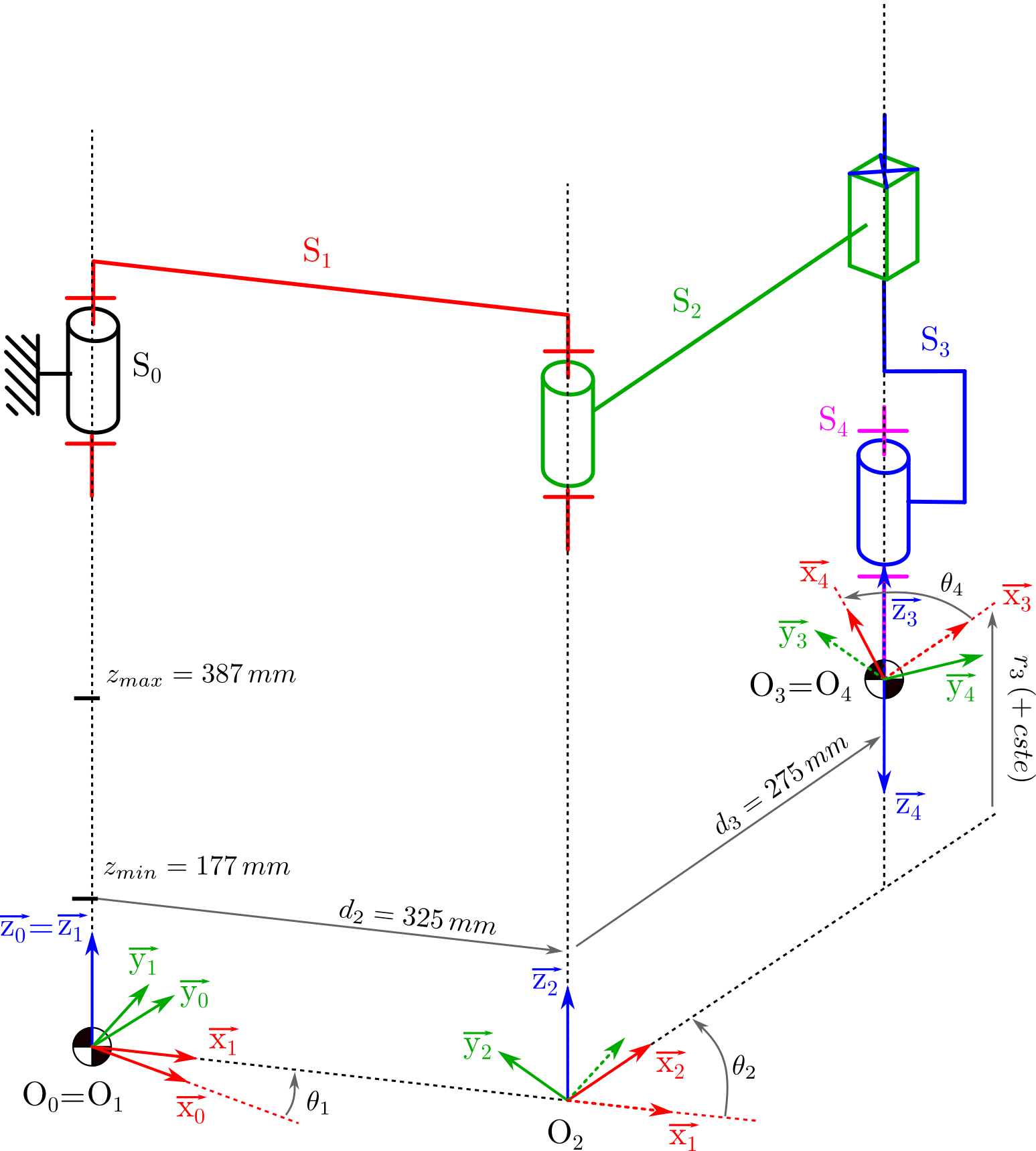
Tableau de paramètres DHm pour le robot

	\(d_i\)	\(\alpha_i\)	\(r_i\)	\(\theta_i\)
\(\mathbf{T}_{01}\)	0	0	0	\(\theta_1\)
\(\mathbf{T}_{12}\)	\(d_2\)	0	0	\(\theta_2\)
\(\mathbf{T}_{23}\)	\(d_3\)	0	\(r_3\, (+ r_{30})\)	0
\(\mathbf{T}_{34}\)	0	\(180^{\circ}\)	0	\(\theta_4\)

Les paramètres \(d_i\) et \(\alpha_i\) sont toujours constants.

Les paramètres \(r_i\) et \(\theta_i\) sont les variables articulaires et sont définies à une constante près.

Question 1.3 : Déterminer chaque matrice homogène de transformation \(\mathbf{T}_{ij}\) entre les différents corps.

Solution

Matrices homogènes élémentaires de transformations entre repères :

\[\begin{split} \begin{align*} \mathbf{T}_{01}&= \begin{bmatrix} \text{C}\theta_1 & -\text{S}\theta_1 & 0 & 0 \\ \text{S}\theta_1 & \text{C}\theta_1 & 0 & 0 \\ 0 & 0 & 1 & 0 \\ 0 & 0 & 0 & 1\\ \end{bmatrix} \\ \\ \mathbf{T}_{12}&= \begin{bmatrix} \text{C}\theta_2 & -\text{S}\theta_2 & 0 & d_2 \\ \text{S}\theta_2 & \text{C}\theta_2 & 0 & 0 \\ 0 & 0 & 1 & 0 \\ 0 & 0 & 0 & 1\\ \end{bmatrix} \\ \\ \mathbf{T}_{23}&= \begin{bmatrix} 1 & 0 & 0 & d_3 \\ 0 & 1 & 0 & 0 \\ 0 & 0 & 1 & r_3 \\ 0 & 0 & 0 & 1\\ \end{bmatrix} \end{align*} \end{split}\]

Pour \(\mathbf{T}_{34}\) : la matrice de rotation \(\mathbf{R}_{34}\) est composée de 2 rotations :

\[\begin{split} \begin{align*} \mathbf{R}_{34} &= \begin{bmatrix} 1 & 0 & 0 \\ 0 & \text{C}(\pi) & -\text{S}(\pi) \\ 0 & \text{S}(\pi) & \text{C}(\pi) \\ \end{bmatrix} \times \begin{bmatrix} \text{C}\theta_4 & -\text{S}\theta_4 & 0 \\ \text{S}\theta_4 & \text{C}\theta_4 & 0 \\ 0 & 0 & 1 \\ \end{bmatrix} \\ \\ \mathbf{R}_{34} &= \begin{bmatrix} \text{C}\theta_4 & -\text{S}\theta_4 & 0 \\ -\text{S}\theta_4 & -\text{C}\theta_4 & 0 \\ 0 & 0 & -1 \\ \end{bmatrix} \end{align*} \end{split}\]

On trouve ainsi :

\[\begin{split} \begin{equation*} \mathbf{T}_{34} = \begin{bmatrix} \text{C}\theta_4 & -\text{S}\theta_4 & 0 & 0 \\ -\text{S}\theta_4 & -\text{C}\theta_4 & 0 & 0 \\ 0 & 0 & -1 & 0 \\ 0 & 0 & 0 & 1\\ \end{bmatrix} \end{equation*} \end{split}\]

Question 1.4 : En déduire l’expression de la transformation globale permettant de passer d’un vecteur exprimé dans le référentiel associé à l’effecteur \(\mathcal{R}_{\text{eff.}}\), à son expression dans le référentiel associé à la base du robot \(\mathcal{R}_0\) :

\[ \begin{equation} {}^0\mathbf{P} = \mathbf{T_{0\,\text{eff}}} \, {}^\text{eff}\mathbf{P} \end{equation} \]

Solution

\[ \begin{equation*} {}^0\mathbf{P} = \mathbf{T}_{01} \, \mathbf{T}_{12} \, \mathbf{T}_{23} \, \mathbf{T}_{34} \, {}^4\mathbf{P} \end{equation*} \]

Calcul de l’expression de \(\mathbf{T}_{04}\). \

1. On commence par calculer le produit \(\mathbf{T}_{23} \times \mathbf{T}_{34}\) car \(\mathbf{T}_{23}\) est seulement une matrice de translation.

   \[\begin{split} \begin{equation*} \mathbf{T}_{24} = \begin{bmatrix} \text{C}\theta_4 & -\text{S}\theta_4 & 0 & d_3 \\ -\text{S}\theta_4 & -\text{C}\theta_4 & 0 & 0 \\ 0 & 0 & -1 & r_3 + cste \\ 0 & 0 & 0 & 1\\ \end{bmatrix} \end{equation*} \end{split}\]

2. Calcul du produit \(\mathbf{T}_{12} \times \mathbf{T}_{24}\)

   \[\begin{split} \begin{align*} \mathbf{T}_{14} &= \begin{bmatrix} \text{C}\theta_2 \text{C}\theta_4 + \text{S}\theta_2 \text{S}\theta_4 & - \text{C}\theta_2 \text{S}\theta_4 + \text{S}\theta_2 \text{C}\theta_4 & 0 & d_3 \text{C}\theta_2 + d_2\\ \text{S}\theta_2 \text{C}\theta_4 - \text{C}\theta_2 \text{S}\theta_4 & - \text{S}\theta_2 \text{S}\theta_4 - \text{C}\theta_2 \text{C}\theta_4 & 0 & d_3 \text{S}\theta_2 \\ 0 & 0 & -1 & r_3 + cste \\ 0 & 0 & 0 & 1\\ \end{bmatrix} \\ \\ &= \begin{bmatrix} \text{C}(\theta_2-\theta_4) & \text{S}(\theta_2-\theta_4) & 0 & d_3 \text{C}\theta_2 + d_2\\ \text{S}(\theta_2-\theta_4) & -\text{C}(\theta_2-\theta_4) & 0 & d_3 \text{S}\theta_2 \\ 0 & 0 & -1 & r_3 + cste \\ 0 & 0 & 0 & 1\\ \end{bmatrix} \end{align*} \end{split}\]

   Rappel trigonométrique $\( \begin{align*} \text{S}(a+b) &= \text{S}(a)\text{C}(b) +\text{C}(a)\text{S}(b) \\ \text{C}(a+b) &= \text{C}(a)\text{C}(b) -\text{S}(a)\text{S}(b) \end{align*} \)$

3. Calcul du produit \(\mathbf{T}_{01} \times \mathbf{T}_{14}\)

   \[\begin{split} \begin{align*} \mathbf{T}_{04} &= \begin{bmatrix} \text{C}\theta_1 \text{C}(\theta_2-\theta_4) - \text{S}\theta_1 \text{S}(\theta_2-\theta_4) & \text{C}\theta_1 \text{S}(\theta_2-\theta_4) + \text{S}\theta_1 \text{C}(\theta_2-\theta_4) & 0 & \text{C}\theta_1 (d_3 \text{C}\theta_2 + d_2) - \text{S}\theta_1 (d_3 \text{S}\theta_2) \\ \text{S}\theta_1 \text{C}(\theta_2-\theta_4) - \text{C}\theta_1 \text{S}(\theta_2-\theta_4) & \text{S}\theta_1 \text{S}(\theta_2-\theta_4) - \text{C}\theta_1 \text{C}(\theta_2-\theta_4) & 0 & \text{S}\theta_1 (d_3 \text{C}\theta_2 + d_2) + \text{C}\theta_1 (d_3 \text{S}\theta_2) \\ 0 & 0 & -1 & r_3 + cste \\ 0 & 0 & 0 & 1\\ \end{bmatrix} \\ \\ &= \begin{bmatrix} \text{C}(\theta_1+\theta_2-\theta_4) & \text{S}(\theta_1+\theta_2-\theta_4) & 0 & d_3 \text{C}(\theta_1 + \theta_2) + d_2 \text{C}\theta_1 \\ \text{S}(\theta_1+\theta_2-\theta_4) & -\text{C}(\theta_1+\theta_2-\theta_4) & 0 & d_3 \text{S}(\theta_1 + \theta_2) + d_2 \text{S}\theta_1 \\ 0 & 0 & -1 & r_3 + cste \\ 0 & 0 & 0 & 1\\ \end{bmatrix} \end{align*} \end{split}\]

Question 1.5 : Retrouver par un raisonnement géométrique simple les équations définissant le vecteur translation entre le repère \(\mathcal{R}_0\) et le repère de l’effecteur \(\mathcal{R}_{\text{eff.}}\).

Solution

Pour retrouver les équations liées à la position de l’effecteur, il suffit de réaliser un schéma dans le plan.

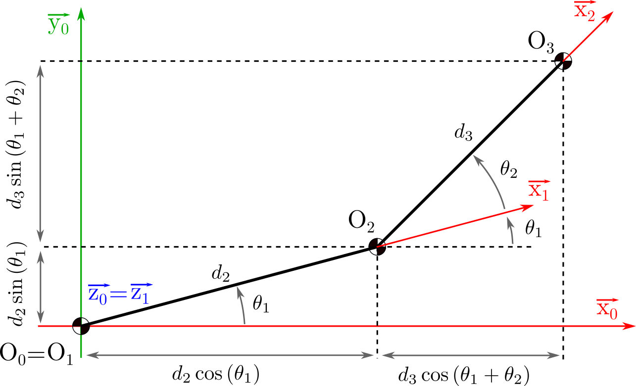
Si on nomme \((x,y,z)\) le vecteur translation entre le repère \(\mathcal{R}_0\) et le repère de l’effecteur \(\mathcal{R}_{\text{eff}}\). On retrouve bien :

\[\begin{split} \begin{equation*} \begin{cases} x = d_3 \text{C}(\theta_1+\theta_2)+d_2 \text{C}\theta_1 \\ y = d_3 \text{S}(\theta_1+\theta_2)+d_2 \text{S}\theta_1 \end{cases} \end{equation*} \end{split}\]

Modélisation Géométrique Directe et Inverse

Question 2.1 : Proposer un paramétrage du repère effecteur \(\mathcal{R}_{\text{eff}}\) par rapport au repère de base \(\mathcal{R}_0\).

Solution

Pour le robot scara la position et l’orientation de l’organe terminal sont caractérisé par :

• 3 composantes pour la position : \(x\), \(y\), \(z\)

• 1 composante pour l’orientation dans le plan : \(\omega\)

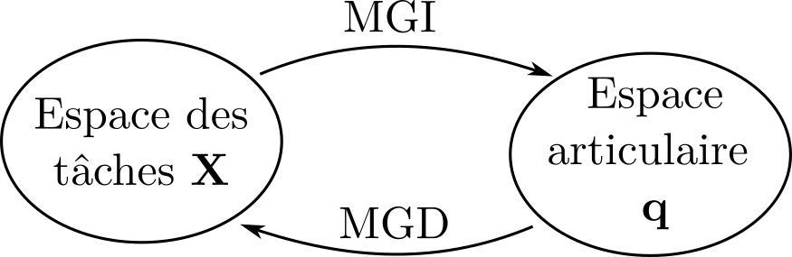
Soit \(\mathbf{X} = (x, y, z, \omega)\) le vecteur contenant les paramètres de l’espace des tâches et \(\mathbf{q} = (\theta_1, \theta_2, r_3, \theta_4)\) le vecteur contenant les paramètres de l’espace articulaire.

Modèle géométrique directe :

\[ \begin{equation*} \mathbf{X} = f_{MGD}(\mathbf{q}) \end{equation*} \]

Modèle géométrique inverse :

\[ \begin{equation*} \mathbf{q} = f_{MGI}(\mathbf{X}) \end{equation*} \]

Question 2.2 : En étudiant successivement le problème en orientation puis en position, exprimer le MGD.

Solution

1 - MGD en orientation :

\[ \begin{equation*} {}^0\mathbf{P} = \mathbf{T}_{04} \, {}^4\mathbf{P} \end{equation*} \]

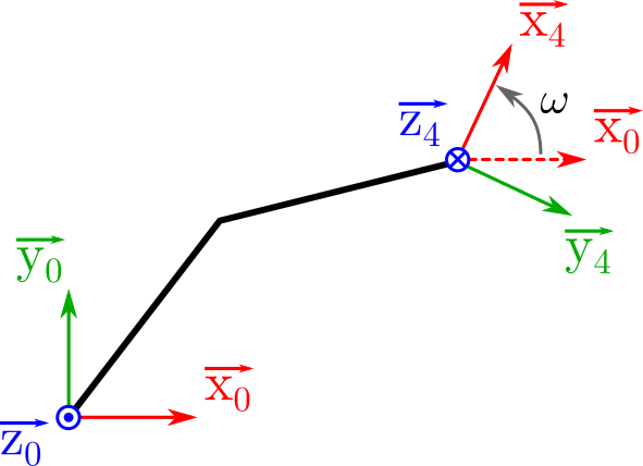
Orientation de \(\overrightarrow{z_4}\) opposé à \(\overrightarrow{z_0}\).\

\(\omega\) correspond à l’angle entre \((\overrightarrow{x_0}, \overrightarrow{x_4})\). On cherche donc a exprimer \(\overrightarrow{x_4}\) dans le repère \(\mathcal{R}_0\)

\[\begin{split} \begin{align*} ^0\overrightarrow{x_4} &= \mathbf{T}_{04} ~^4\overrightarrow{x_4} \\ &= \mathbf{T}_{04} \begin{pmatrix} 1 \\ 0 \\ 0 \\ 0 \end{pmatrix} \\ &= \begin{pmatrix} \cos(\theta_1 + \theta_2 - \theta_4) \\ \sin(\theta_1 + \theta_2 - \theta_4) \\ 0 \\ 0 \\ \end{pmatrix} \end{align*} \end{split}\]

Par identification de l’expression de \(\overrightarrow{x_4}\) exprimé dans le repère \(\mathcal{R}_0\) on trouve :

\[ \begin{equation*} \omega = \theta_1 + \theta_2 - \theta_4 \end{equation*} \]

2 - MGD en position :

On détermine les coordonnées de \(O_4\) dans le repère \(\mathcal{R}_0\)

\[\begin{split} \begin{equation*} \begin{pmatrix} x \\ y \\ z \\ 1 \end{pmatrix} = \mathbf{T}_{04} \begin{pmatrix} 0 \\ 0 \\ 0 \\ 1 \end{pmatrix} \end{equation*} \end{split}\]

On trouve ainsi le MGD :

\[\begin{split} \begin{equation*} \begin{cases} \omega = \theta_1 + \theta_2 - \theta_4 \qquad \qquad \qquad \, \, (1) \\ x = d_3 \text{C}(\theta_1+\theta_2)+d_2 \text{C}\theta_1 \qquad (2) \\ y = d_3 \text{S}(\theta_1+\theta_2)+d_2 \text{S}\theta_1 \qquad \, \, \, (3) \\ z = r_3 + cste \qquad \qquad \qquad \quad \, \, \, \, \, \,(4) \end{cases} \end{equation*} \end{split}\]

Question 2.3 : A l’aide des formulations géométriques données en Annexe des « Notes de cours » , exprimer le MGI.

Solution

• 1 - Déterminer \(\theta_1\) et \(\theta_2\) en fonction de \(x\) et \(y\)

• 2 - Déterminer \(\theta_4\) permettant de réaliser \(\omega\) étant donnés \(\theta_1\) et \(\theta_2\) imposés

Le système d’équation suivant correspond à un système de type 8 (notes de cours) :

\[\begin{split} \begin{equation*} \begin{cases} x = d_3 \text{C}(\theta_1+\theta_2)+d_2 \text{C}\theta_1 \\ y = d_3 \text{S}(\theta_1+\theta_2)+d_2 \text{S}\theta_1 \\ \end{cases} \end{equation*} \end{split}\]

2 solutions (cf. démonstration en annexe) :

\[ \begin{equation*} \theta_2 = \text{atan2} \left( \pm \sqrt{1-\cos^2(\theta_2)},\cos(\theta_2) \right) \quad \text{avec} \quad \cos(\theta_2) = \dfrac{x^2+y^2-d_2^2-d_3^2}{2 d_2 d_3} \end{equation*} \]

\[\begin{split} \begin{equation*} \theta_1 = \text{atan2} \left(\sin(\theta_1),\cos(\theta_1)\right) \quad \text{avec} \quad \begin{cases} \cos(\theta_1) = \dfrac{x B_1 + y B_2}{B_1^2 + B_2^2} \\ \sin(\theta_1) = \dfrac{y B_1 - x B_2}{B_1^2 + B_2^2} \end{cases} \quad \text{avec} \quad \begin{cases} B_1 = d_2 + d_3 \cos(\theta_2) \\ B_2 = d_3 \sin(\theta_2) \end{cases} \end{equation*} \end{split}\]

Ensuite, une fois \(\theta_1\) et \(\theta_2\) résolus, on peut déterminer \(\theta_4\).

\[ \begin{equation*} \theta_4 = \theta_1 + \theta_2 - \omega \end{equation*} \]

La dernière relation est évidente :

\[ \begin{equation*} r_3 = z - cste \end{equation*} \]

On trouve ainsi le MGI :

\[\begin{split} \begin{equation*} \begin{cases} \theta_2 = \text{atan2} \left( \pm \sqrt{1-\cos^2(\theta_2)},\cos(\theta_2) \right) \quad \text{avec} \quad \cos(\theta_2) = \dfrac{x^2+y^2-d_2^2-d_3^2}{2 d_2 d_3} \\ \theta_1 = \text{atan2} \left(\sin(\theta_1),\cos(\theta_1)\right) \quad \text{avec} \quad \begin{cases} \cos(\theta_1) = \dfrac{x B_1 + y B_2}{B_1^2 + B_2^2} \\ \sin(\theta_1) = \dfrac{y B_1 - x B_2}{B_1^2 + B_2^2} \end{cases} \quad \text{avec} \quad \begin{cases} B_1 = d_2 + d_3 \cos(\theta_2) \\ B_2 = d_3 \sin(\theta_2) \end{cases} \\ \theta_4 = \theta_1 + \theta_2 - \omega) \\ r_3 = z - cste \end{cases} \end{equation*} \end{split}\]

Synthèse

Question 3.1 : Analyser le modèle du robot implémenté dans l’application « RoboDK ».

Solution

RoboDK : Logiciel permettant de simuler pour différents robots, différentes trajectoires.

1. Ouvrir la librairie en ligne (icône avec la planète). De nombreux robot dont le robots à architecture Scara utilisé dans ce TP sont disponibles.

2. Ouvrir le robot Scara utilisé dans le TP. Par défaut, on a directement le repère de référence qui s’affiche et le repère de l’organe terminal. Correspondance des couleurs (X -> rouge, Y -> vert, Z -> bleu)

3. Double clic sur le robot pour faire apparaitre la fenêtre des propriétés.

   • Expliquer les différentes sous-parties disponibles.

   • Décoché tous les repères

   • Faire apparaitre le repère 1 et le repère 2, faire varier l’angle \(\theta_1\) et l’angle \(\theta_2\). Comme vu précédemment on peut placer les origines au même endroit : il n’y a qu’un paramètre \(d_1\) qui apparait.

   • Faire le lien avec la variation des paramètres que l’on a dans les différents repères : Attention les notations ne sont pas les mêmes

4. Montrer les autres configurations possibles : Attention il n’y a pas 4 configurations, mais seulement 2 : la variation de \(\theta_4\) n’est pas entre \(-360\deg\) et \(360\deg\) mais uniquement entre \(0\deg\) et \(360\deg\) (1 seul tour possible).

5. Montrer l’espace de travail complet que l’on peut obtenir.

6. Cliquer sur paramètres en haut à droite afin d’accéder au modèle géométrique du robot : Attention, les paramètres géométriques sont décrits au sens du modèle de Denavit Hartenberg (DH) et non au sens de Denavit Hartenberg modifié (DHm)

Annexes

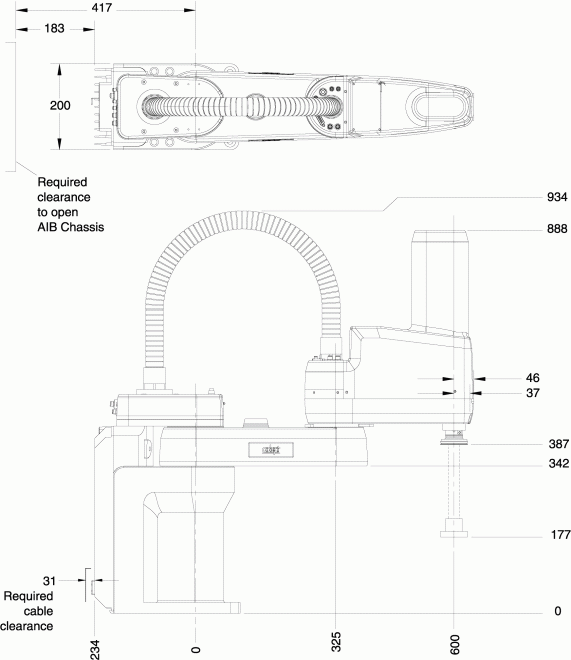
Fig. 29 Caractéristiques dimensionnelles

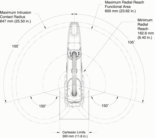
Fig. 30 Surface balayée par l’effecteur

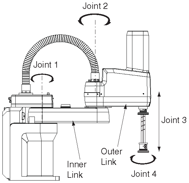
Fig. 31 Extrait de documentation : cinématique

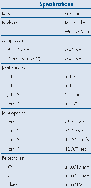
Fig. 32 Extrait de documentation : spécifications

Solution

Démonstration des solutions de l’équation de type 8 :

Le système a résoudre est le suivant :

\[\begin{split} \begin{equation*} \begin{cases} x = d_3 \text{C}(\theta_1+\theta_2)+d_2 \text{C}\theta_1 \\ y = d_3 \text{S}(\theta_1+\theta_2)+d_2 \text{S}\theta_1 \\ \end{cases} \end{equation*} \end{split}\]

par identification au cours on a \(\theta_1 = \theta_i\), \(\theta_2 = \theta_j\), \(d_2 = X\), \( d_3 = Y\), \(x = Z_1\) et \(y = Z_2\).

L’équation générique est donc :

\[\begin{split} \begin{equation*} \begin{cases} X \text{C}\theta_i + Y \text{C}(\theta_i+\theta_j) = Z_1 \\ X \text{S}\theta_i + Y \text{S}(\theta_i+\theta_j) = Z_2\\ \end{cases} \end{equation*} \end{split}\]

Résolution pour trouver \(\theta_j\)

On élève au carré les deux équations et on additionne :

\[ \begin{equation*} X^2 \text{C}^2(\theta_i) + X^2 \text{S}^2(\theta_i) + Y^2 \text{C}^2(\theta_i + \theta_j) + Y^2 \text{S}^2(\theta_i + \theta_j) + 2 X Y \underbrace{\left[ \text{C}(\theta_i)\text{C}(\theta_i+\theta_j) + \text{S}(\theta_i)\text{S}(\theta_i+\theta_j) \right]}_{\text{C}(\theta_i+\theta_j-\theta_i) \, \, \text{ou} \, \, \text{C}(\theta_i - (\theta_i+\theta_i))} = Z_1^2 + Z_2^2 \end{equation*} \]

La partie avec une accolade correspond soit à \(\cos(\theta_j)\) soit à \(\cos(-\theta_j)\). On utilise la propriété du \(\text{C}^2(a) + \text{S}^2(a) = 1\) pour simplifier l’équation précédente. On trouve donc :

\[ \begin{equation*} \cos(\theta_j) = \dfrac{Z_1^2 + Z_2^2 - X^2 -Y^2}{2 X Y } \quad \text{et} \quad \sin(\theta_j) = \sqrt{1 - \cos(\theta_j)} \end{equation*} \]

d’ou :

\[\begin{split} \begin{equation*} \theta_j = \text{atan2} \left( \pm \sqrt{1 - \cos^2(\theta_j)}, \cos(\theta_j) \right) \end{equation*} \\ \end{split}\]

Résolution pour trouver \(\theta_i\)

Développement du \(\cos(a+b)\) et \(\sin(a+b)\)

\[\begin{split} \begin{equation*} \begin{cases} X \text{C}\theta_i + Y \left(\text{C}\theta_i \text{C}\theta_j -\text{S}\theta_i \text{S}\theta_j \right)= Z_1 \\ X \text{S}\theta_i + Y \left(\text{S}\theta_i \text{C}\theta_j +\text{C}\theta_i \text{S}\theta_j \right)= Z_2\\ \end{cases} \end{equation*} \end{split}\]

\[\begin{split} \begin{equation*} \begin{cases} \text{C}\theta_i \left[X+ Y \text{C} \theta_j \right] + \text{S}\theta_i \left[ - Y \text{S}\theta_j \right] = Z_1 \\ \text{C}\theta_i \left[ Y \text{S}\theta_j\right] + \text{S}\theta_i \left[X+ Y \text{C} \theta_j \right] = Z_2 \end{cases} \end{equation*} \end{split}\]

On note \(B_1 = Y \text{S}\theta_j\) et \(B_2 = X+ Y \text{C} \theta_j\). On obtient le système suivant que l’on note \((S1)\)

\[\begin{split} \begin{equation*} \begin{cases} \text{C}\theta_i B_1 - \text{S}\theta_i B_2 = Z_1 \\ \text{C}\theta_i B_2 + \text{S}\theta_i B_1 = Z_2 \end{cases} \end{equation*} \end{split}\]

1. On multiplie la première équation de \((S1)\) par \(B_2\) et la seconde par \(B_1\). On obtient :

   \[\begin{split} \begin{equation*} \begin{cases} \text{C}\theta_i B_1 B_2 - \text{S}\theta_i B_2^2 = Z_1 B_2 \qquad (1)\\ \text{C}\theta_i B_1 B_2 + \text{S}\theta_i B_1^2 = Z_2 B_1 \qquad (2) \end{cases} \end{equation*} \end{split}\]

   En soustrayant l’équation \((1)\) à l’équation \((2)\) on obtient :

   \[ \begin{equation*} \text{S}\theta_i (B_1^2 + B_2^2) = Z_2 B_1 - Z_1 B_2 \end{equation*} \]

   d’ou :

   \[ \begin{equation*} \text{S}\theta_i = \dfrac{Z_2 B_1 - Z_1 B_2}{B_1^2 + B_2^2} \qquad \text{avec} \qquad B_1^2 + B_2^2 \ne 0 \end{equation*} \]

2. On multiplie la première équation de \((S1)\) par \(B_1\) et la seconde par \(B_2\). On obtient :

   \[\begin{split} \begin{equation*} \begin{cases} \text{C}\theta_i B_1^2 - \text{S}\theta_i B_2 B_1 = Z_1 B_1 \qquad (3)\\ \text{C}\theta_i B_2^2 + \text{S}\theta_i B_1 B_2 = Z_2 B_2 \qquad (4) \end{cases} \end{equation*} \end{split}\]

   En additionnant l’équation \((3)\) et \((4)\) on obtient :

   \[ \begin{equation*} \text{C}\theta_i = \dfrac{Z_1 B_1 + Z_2 B_2}{B_1^2 + B_2^2} \qquad \text{avec} \qquad B_1^2 + B_2^2 \ne 0 \end{equation*} \]

Maintenant que l’on a connaisance de \(\cos(\theta_i)\) et \(\sin(\theta_i)\) on peu dire :

\[ \begin{equation*} \theta_i = \text{atan2}( \text{S}\theta_i, \text{C}\theta_i) \end{equation*} \]