Correction du TD n°3 : Modélisations cinématiques - Singularités

On étudie le robot Scara 4 axes, référencé « s600 » de marque Adept donné en Fig. 44 :

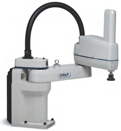
Fig. 44 Robot SCARA s600

Pour cette étude, on tiendra pas compte des courses de chaque axe afin de ne pas être limité dans les mouvements ; on négligera de même les potentielles collisions.

Modélisations cinématiques

Calcul analytique

Question 1.1 : A partir du schéma cinématique et du paramétrage DHm effectué au TD n°1, déterminer les expressions des vecteur rotation et vecteur vitesse du référentiel associé à l’effecteur \(\mathcal{R}_{\text{eff.}}\) dans son mouvement par rapport au référentiel de base \(\mathcal{R}_0\).

On utilisera préférentiellement la composition du mouvement et la relation de changement de point pour le calcul du vecteur vitesse.

Solution

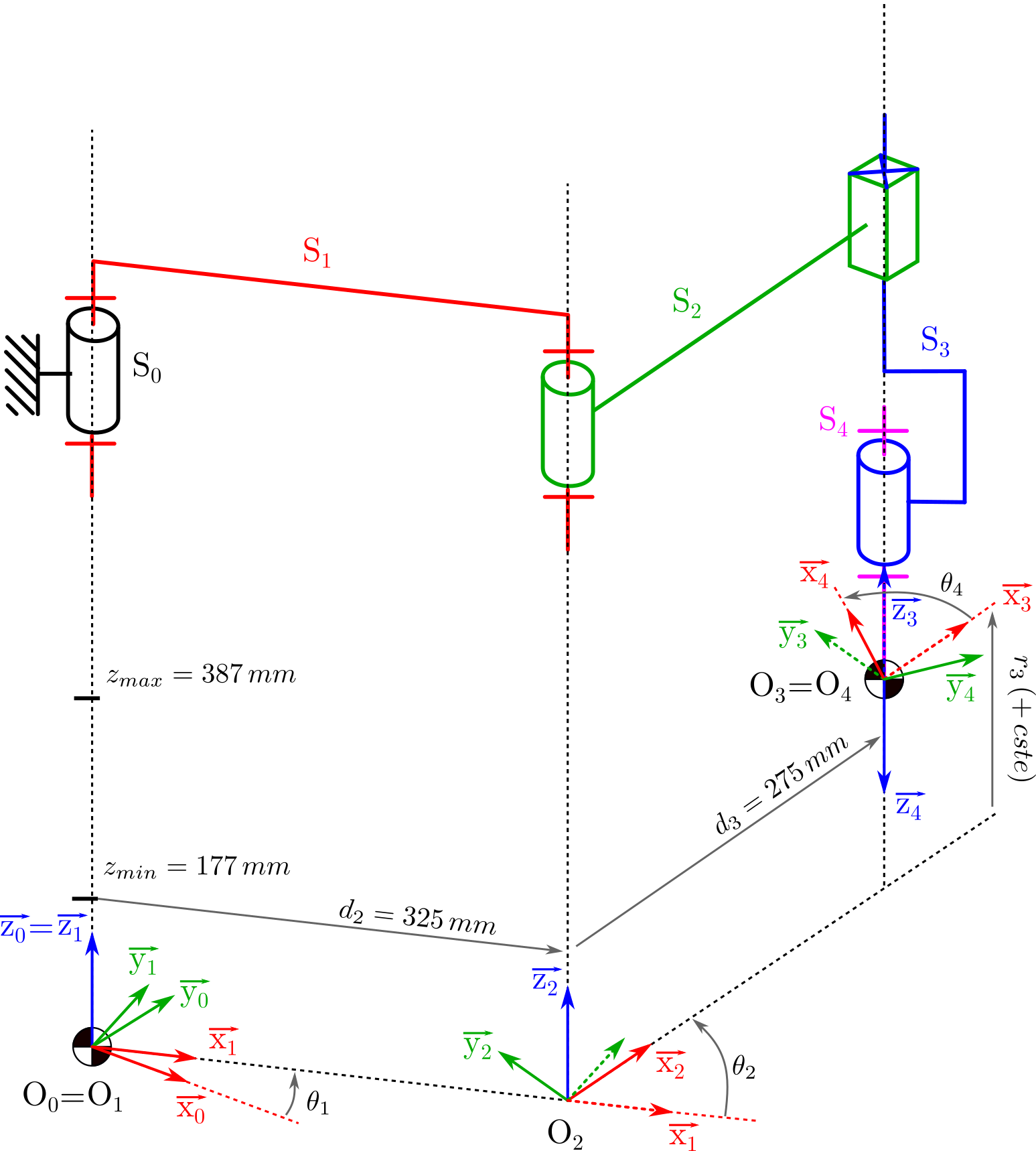
Le paramétrage du robot Scara tel qu’il a été effectué dans le TD1 est proposé en annexe.

On cherche \(\overrightarrow{V_{O_4 \in 4/0}}\) et \(\overrightarrow{\Omega_{4/0}}\)

1 - Vecteur vitesse :

\[\begin{split} \begin{align*} \overrightarrow{V_{O_4 \in 4/0}} &= \overrightarrow{V_{O_3 \in 3/0}} \quad \text{car} \quad O_4 = O_3 \quad \text{et} \quad O_3 \in \text{axe rotation 3/4} \\ &= \overrightarrow{V_{O_3 \in 3/2}} + \overrightarrow{V_{O_3 \in 2/0}} \\ &= \dot{r_3} \overrightarrow{z}_0 + \overrightarrow{V_{O_2 \in 2/0}} + \overrightarrow{\Omega_{2/0}} \wedge \overrightarrow{O_2 O_3} \\ &= \dot{r_3} \overrightarrow{z}_0 + \overrightarrow{V_{O_2 \in 2/1}} + \overrightarrow{V_{O_2 \in 1/0}} + \overrightarrow{\Omega_{2/0}} \wedge \overrightarrow{O_2 O_3} \\ &= \dot{r_3} \overrightarrow{z}_0 + \overrightarrow{V_{O_2 \in 2/1}} + \overrightarrow{V_{O_1 \in 1/0}} + \overrightarrow{\Omega_{1/0}} \wedge \overrightarrow{O_1 O_2} + \overrightarrow{\Omega_{2/0}} \wedge \overrightarrow{O_2 O_3} \end{align*} \end{split}\]

\( \overrightarrow{V_{O_2 \in 2/1}} = 0 \text{ car } O_2 \in \text{ axe } 2/1 \quad \text{ et } \quad \overrightarrow{V_{O_1 \in 1/0}} = 0 \text{ car } O_1 \in \text{ axe } 1/0 \)

\[\begin{split} \begin{align*} &= \dot{r_3} \overrightarrow{z}_0 + \overrightarrow{\Omega_{1/0}} \wedge \overrightarrow{O_1 O_2} + \overrightarrow{\Omega_{2/0}} \wedge \overrightarrow{O_2 O_3} \\ &= \dot{r_3} \overrightarrow{z}_0 + \dot{\theta_1} \overrightarrow{z}_0 \wedge (d_2 \overrightarrow{x_1}) + (\dot{\theta_1}+\dot{\theta_2})\overrightarrow{z}_0 \wedge (d_3 \overrightarrow{x_2}-r_3 \overrightarrow{z}_0 ) \\ \overrightarrow{V_{O_4 \in 4/0}} &= \dot{r_3} \overrightarrow{z}_0 + d_2 \dot{\theta_1} \overrightarrow{y_1} + d_3 (\dot{\theta_1}+\dot{\theta_2})\overrightarrow{y_2} \end{align*} \end{split}\]

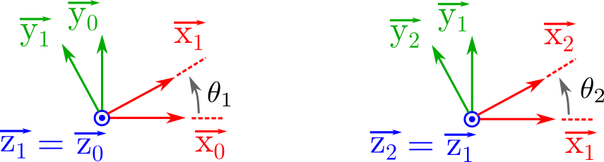
En utilisant les figures de changement de repère on exprime \(\overrightarrow{V_{O_4 \in 4/0}}\) dans le repère \(\mathcal{R}_0\).

\[ \begin{align*} \overrightarrow{V_{O_4 \in 4/0}} = \dot{r_3}\overrightarrow{z}_0 + \left[ -d_2 \dot{\theta_1} \sin(\theta_1) - d_3 (\dot{\theta_1}+\dot{\theta_2}) \sin(\theta_1+\theta_2) \right] \overrightarrow{x_0} + \left[ d_2 \dot{\theta_1} \cos(\theta_1) + d_3 (\dot{\theta_1}+\dot{\theta_2}) \cos(\theta_1+\theta_2)\right] \overrightarrow{y_0} \end{align*} \]

2 - vecteur taux de rotation :

\[\begin{split} \begin{align*} \overrightarrow{\Omega_{4/0}} &= \overrightarrow{\Omega_{4/3}} + \overrightarrow{\Omega_{3/2}} + \overrightarrow{\Omega_{2/1}} + \overrightarrow{\Omega_{1/0}} \\ &= (\dot{\theta_4}+\dot{\theta_2}+\dot{\theta_1}) \overrightarrow{z}_0 \end{align*} \end{split}\]

Question 1.2 : En déduire l’expression de la matrice jacobienne \(\mathbf{J}\) et donc le Modèle Cinématique Direct (MCD).

Solution

Il suffit d’exprimer sous forme matricielle \(\dot{\mathbf{X}} = \mathbf{J} (\mathbf{Q}) \cdot \dot{\mathbf{Q}}\) :

\[\begin{split} \begin{equation*} \mathbf{J} (\theta_1, \theta_2, r_3, \theta_4) = \begin{pmatrix} 1 & 1 & 0 & -1 \\ - d_2 \text{S}\theta_1 - d_3 \text{S}(\theta_1 + \theta_2) & - d_3 \text{S}(\theta_1 + \theta_2 & 0 & 0 \\ d_2 \text{C}\theta_1 + d_3 \text{C}(\theta_1 + \theta_2) & d_3 \text{C}(\theta_1 + \theta_2 & 0 & 0 \\ 0 & 0 & 1 & 0 \\ \end{pmatrix} \end{equation*} \end{split}\]

La Jacobienne dépend de la configuration du robot (ici seulement de \(\theta_1\) et \(\theta_2\)).

Attention le résultat n’est en aucun cas une matrice homogène ! ne pas confondre. Ici on à 4 colonnes représentant la dérivé temporelle des 4 paramètres articulaires \(\dot{\mathbf{Q}} = (\dot{\theta_1}, \dot{\theta_2}, \dot{r_3}, \dot{\theta_4}) \) et 4 lignes représentant les dérivées temporelles des 4 paramètres définissant la position et l’orientation de l’effecteur dans l’espace des tâches \(\dot{\mathbf{X}} = (\dot{\omega}, \dot{x}, \dot{y}, \dot{z})\).

Différentiation - dérivation

Question 1.3 : Retrouver rapidement le résultat précédent par dérivation du Modèle Géométrique Direct établi au TD n°1.

Solution

MGD trouvé au TD n°1 :

\[\begin{split} \begin{equation*} \begin{cases} \omega = \theta_1 + \theta_2 - \theta_4 \\ x = d_3 \cos(\theta_1+\theta_2)+d_2 \cos\theta_1 \\ y = d_3 \sin(\theta_1+\theta_2)+d_2 \sin\theta_1 \\ z = r_3 + cste \end{cases} \end{equation*} \end{split}\]

Dérivation du MGD :

\[\begin{split} \begin{equation*} \begin{cases} \dot{\omega} = \dot{\theta_1} + \dot{\theta_2} - \dot{\theta_4} \\ \dot{x} = - d_3 \sin(\theta_1+\theta_2)(\dot{\theta_1}+\dot{\theta_2})-d_2 \sin(\theta_1) \dot{\theta} \\ \dot{y} = - d_3 \cos(\theta_1+\theta_2)(\dot{\theta_1}+\dot{\theta_2})+d_2 \cos(\theta_1) \dot{\theta} \\ \dot{z} = \dot{r_3} \end{cases} \end{equation*} \end{split}\]

La dérivation du MGD nous permet d’obtenir le mêm résultat que précédemment. Dans le cas ou la structure du robot est complexe, on préférera calculer par la cinématique.

Jacobien de base

Question 1.4 : Déterminer le jacobien de base \(\mathbf{J}_n\) à partir des contributions de chaque liaison \(\mathbf{J}_{n,k}\).

Solution

\[ \begin{equation*} ^0 \dot{\mathbf{X}} = \mathbf{\Omega}\cdot ^0 \dot{\mathbf{J_n}} \cdot \dot{\mathbf{Q}} \end{equation*} \]

\(\mathbf{\Omega}\) est une fonction du paramétrage.

Rappel : Le jacobien de base représente la contribution de l’articulation (liaison) à la vitesse du référentiel extrémité. \(k\) désigne la k-ième liaison

\[\begin{split} \begin{equation*} \text{Pivot :} \qquad J_{n,k} = \begin{pmatrix} \overrightarrow{z_k} \\ \overrightarrow{L_{k,n}} \wedge \overrightarrow{z_k} \end{pmatrix} \qquad \text{Glissière :} \qquad J_{n,k} = \begin{pmatrix} \overrightarrow{0} \\ \overrightarrow{z_k} \end{pmatrix} \end{equation*} \end{split}\]

Ici on a un robot a 4 axes donc 4 jacobien de base élémentaires (3 rotations + 1 translation).

\[\begin{split} \begin{equation*} J_{4,1} = \begin{pmatrix} \overrightarrow{z}_0 \\ \overrightarrow{O_4 O_1} \wedge \overrightarrow{z}_0 \end{pmatrix} \qquad J_{4,2} = \begin{pmatrix} \overrightarrow{z}_0 \\ \overrightarrow{O_4 O_2} \wedge \overrightarrow{z}_0 \end{pmatrix} \qquad J_{4,3} = \begin{pmatrix} \overrightarrow{0} \\ \overrightarrow{z}_0 \end{pmatrix} \qquad J_{4,4} = \begin{pmatrix} \overrightarrow{-z_0 } \\ \underbrace{\overrightarrow{O_4 O_4} \wedge \overrightarrow{z}_0 }_{= \overrightarrow{0}} \end{pmatrix} \end{equation*} \end{split}\]

\[\begin{split} \begin{align*} \overrightarrow{O_4O_1} \wedge \overrightarrow{z}_0 &= (\overrightarrow{O_4O_3}+\overrightarrow{O_3O_2}+\overrightarrow{O_2O_1}) \wedge \overrightarrow{z}_0 \\ &= \overrightarrow{O_4O_3} \wedge \overrightarrow{z}_0 + (- d_3 \overrightarrow{x_2} - d_2 \overrightarrow{x_1}) \wedge \overrightarrow{z}_0 \\ &= \overrightarrow{0} + d_3 \overrightarrow{y_2} + d_2 \overrightarrow{y_1} \\ &= (- d_3 \sin(\theta_1+\theta_2) - d_2 \sin(\theta_1))\overrightarrow{x_0} + ( d_3 \cos(\theta_1+\theta_2) + d_2 \cos(\theta_1))\overrightarrow{y_0} \end{align*} \end{split}\]

\[\begin{split} \begin{align*} \overrightarrow{O_4O_2} \wedge \overrightarrow{z}_0 &= (\overrightarrow{O_4O_3}+\overrightarrow{O_3O_2}) \wedge \overrightarrow{z}_0 \\ &= \overrightarrow{0} - d_3 \overrightarrow{x_2} \wedge \overrightarrow{z}_0 \\ &= d_3 \overrightarrow{y_2} \\ &= - d_3 \sin(\theta_1+\theta_2)\overrightarrow{x_0} + d_3 \cos(\theta_1+\theta_2)v\overrightarrow{y_0} \end{align*} \end{split}\]

d’ou \(J_4 = \left(J_{4,1}, J_{4,2}, J_{4,3}, J_{4,4} \right)\). L’ordre des jacobiens de base dépend du vecteur \(\dot{\mathbf{Q}}\). Ici le jacobien de base correspond directement à la matrice Jacobienne J car le robot est simple et paramétré directement.

\[\begin{split} \begin{equation*} \mathbf{J_n} = \begin{pmatrix} 1 & 1 & 0 & -1 \\ - d_2 \text{S}\theta_1 - d_3 \text{S}(\theta_1 + \theta_2) & - d_3 \text{S}(\theta_1 + \theta_2 & 0 & 0 \\ d_2 \text{C}\theta_1 + d_3 \text{C}(\theta_1 + \theta_2) & d_3 \text{C}(\theta_1 + \theta_2 & 0 & 0 \\ 0 & 0 & 1 & 0 \\ \end{pmatrix} \end{equation*} \end{split}\]

\(\overrightarrow{\Omega}\) que sur \(\overrightarrow{z}_0 \) dans le cas de ce robot. Les lignes représentent le paramétrage \(^0 \omega_4\) et \( ^0 V_4\). Les colonnes représentes la dérivée temporelle des variables articulaires.

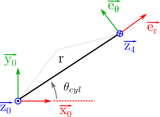
On se donne maintenant comme variables de l’espace des tâches les composantes dans un système de coordonnées cylindriques (au lieu du système cartésien classique).

Question 1.5 : Déterminer l’expression de la matrice \(\mathbf{\Omega}\), lien entre le jacobien de base \(\mathbf{J}_n\) et les variables de l’espace des tâches pour la cinématique \(\dot{\mathbf{X}}\).

Solution

La matrice \(\mathbf{\Omega}\) permet de faire le lien entre différents paramétrages.

Coordonnées cylindrique \(r \cdot \overrightarrow{e_r}\), \(\theta_{cyl}\) et \(z \cdot \overrightarrow{e_z}\).

(24)\[\begin{split} \begin{equation} \begin{cases} x = r \cdot \cos(\theta_{cyl}) \\ y = r \cdot \sin(\theta_{cyl}) \\ z = z \\ \end{cases} \end{equation} \end{split}\]

Inversion du paramétrage

\[\begin{split} \begin{equation*} \begin{cases} r = \sqrt{x^2 + y^2}\\ \theta_{cyl} = \text{atan2}(y,x)\\ z = z \\ \end{cases} \end{equation*} \end{split}\]

il est souvent plus simple de déterminer \(\mathbf{\Omega}\) a partir du système d’équation (24)

\[\begin{split} \begin{equation} \begin{pmatrix} \dot{X_r} \\ \\ \dot{X_p} \\ \\ \end{pmatrix} = \begin{pmatrix} \Omega_r & 0 & 0 & 0 \\ 0 & & & \\ 0 & & \Omega_p & \\ 0 & & & \\ \end{pmatrix} = \begin{pmatrix} ^0 \omega_4 \\ \\ ^0 V_4 \\ \\ \end{pmatrix} \end{equation} \end{split}\]

Le vecteur \((^0 \omega_4, ^0 V_4)\) correspond ici au vecteur \((\dot{\omega}, \dot{x}, \dot{y}, \dot{z})\)

1 - rotation : \(\dot{X_r} = \Omega_r \times ^0 \omega_4\) Or ici le paramétrage en coordonnée cylindrique ne change pas le paramétrage en orientation d’ou : \(\Omega_r = 1\)

2 - translation :

\[ \begin{equation} r = \sqrt{x^2 + y^2} \quad \text{donc} \quad \dot{r} = \dfrac{1}{2} \sqrt{x^2 + y^2} \cdot (2 x \dot{x}+ 2 y \dot{y}) \end{equation} \]

Attention au calcul de la diférentielle de \(\text{atan2}(y,x)\)

\[ \theta_{cyl} = \text{atan2}(y,x) \]

\[\begin{split} \begin{align*} d \theta_{cyl} &= \dfrac{\partial \text{atan2}(y,x)}{\partial x} dx + \dfrac{\partial \text{atan2}(y,x)}{\partial y} dy \\ &= - \dfrac{y}{x^2 +y^2} dx + \dfrac{x}{x^2 +y^2} dy \end{align*} \end{split}\]

d’ou la matrice \(\mathbf{\Omega}\)

\[\begin{split} \begin{equation*} \mathbf{\Omega} = \begin{pmatrix} 1 & 0 & 0 & 0 \\ 0 & \dfrac{X}{\sqrt{X^2+Y^2}} & \dfrac{Y}{\sqrt{X^2+Y^2}} & 0 \\ 0 & - \dfrac{Y}{\sqrt{X^2+Y^2}} & \dfrac{X}{\sqrt{X^2+Y^2}} & 0 \\ 0 & 0 & 0 & 1 \\ \end{pmatrix} \end{equation*} \end{split}\]

Les lignes de la matrice représentent le nouveau paramétrage dans l’espace des taches \(\mathbf{X_{cyl}} = (\dot{\theta}, \dot{r}, \dot{\theta_{cyl}}, \dot{z})\).

Recherche des singularités

Question 2.1 : A partir de l’étude de la jacobienne \(\mathbf{J}\), déterminer les singularités pour ce robot.

Solution

Les singularités correspondent aux valeurs articulaires pour lesquelles le déterminant de la jacobienne est nulle.

\[\begin{split} \begin{equation*} \exists \, \mathbf{Q} \in \mathbb{R}^n \, / \, \det(\mathbf{J}(\mathbf{Q})) = 0 \qquad \text{avec} \qquad \mathbf{J} = \begin{pmatrix} 1 & 1 & 0 & -1 \\ - d_2 \text{S}\theta_1 - d_3 \text{S}(\theta_1 + \theta_2) & - d_3 \text{S}(\theta_1 + \theta_2) & 0 & 0 \\ d_2 \text{C}\theta_1 + d_3 \text{C}(\theta_1 + \theta_2) & d_3 \text{C}(\theta_1 + \theta_2) & 0 & 0 \\ 0 & 0 & 1 & 0 \\ \end{pmatrix} \end{equation*} \end{split}\]

\[\begin{split} \begin{align*} \det \mathbf{J} &= (-1)\times (-1)^{1+4} \det( M_{3\times3}) = \det( M_{3\times3}) \\ &= (1)^{3+3} \det(N_{2\times2}) = \det(N)\\ &= - (d_2 \text{S}\theta_1 + d_3 \text{S}(\theta_1 + \theta_2))(d_3 \text{C}(\theta_1 + \theta_2)) + (d_3 \text{S}(\theta_1 + \theta_2))(d_2 \text{C}\theta_1 + d_3 \text{C}(\theta_1 + \theta_2)) \\ &= -d_2 d_3 \text{S}\theta_1 \text{C}(\theta_1 + \theta_2) + d_2 d_3 \text{C}\theta_1 \text{S}(\theta_1 + \theta_2) \end{align*} \end{split}\]

\[\begin{split} \begin{align*} \det \mathbf{J} = 0 \, &\iff \, \text{S}\theta_1 \text{C}(\theta_1 + \theta_2) - \text{C}\theta_1 \text{S}(\theta_1 + \theta_2) = 0 \\ &\iff \, \text{S}(\theta_1 - (\theta_1 + \theta_2)) = 0 \\ &\iff \, \text{S}(-\theta_2) = 0 \\ &\iff \, \theta_2 = 0 \, \left[ \pi \right] \quad \text{et ce } \quad \forall \theta_1 \in \mathbb{R} \end{align*} \end{split}\]

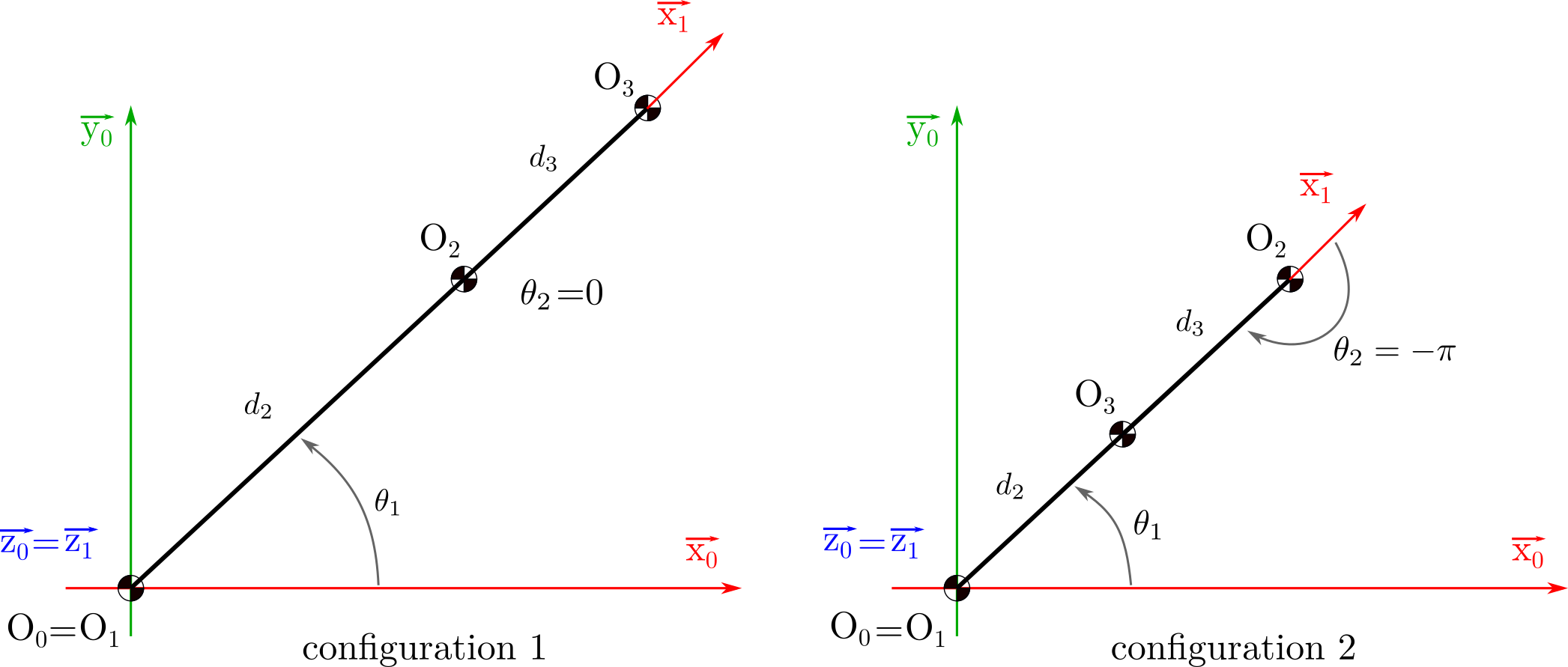
Question 2.2 : Représenter sur un schéma cinématique les différents cas rencontrés ; Expliquer les singularités.

Solution

Les figures suivantes représentent 2 configurations différentes présentant des singularités. Dans la première configuration, il y a une incapacité a généré un mouvement selon \(\overrightarrow{x_1}\), dans la seconde, une incapacité a généré un mouvement selon \(- \overrightarrow{x_1}\).

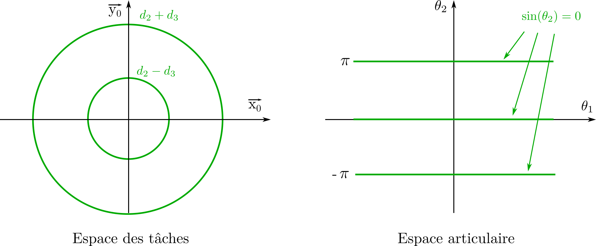
Question 2.3 : Représenter les branches de singularités dans l’espace des tâches et dans l’espace articulaire.

Solution

Les figures suivantes présentent la position des singularités dans les deux espaces :

Synthèse

Analyser le modèle du robot implémenté dans l’application « RoboDK ». Pour cela,

• modifier le paramétrage du robot pour éviter tout problème lié aux courses ;

• positionner le robot dans sa configuration singulière « repliée » ;

• solliciter le robot par des translations « tangentes au rayon » (attention au pas de calcul).

Annexes

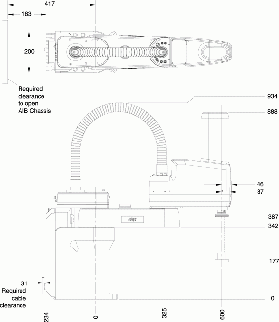
Fig. 45 Caractéristiques dimensionnelles

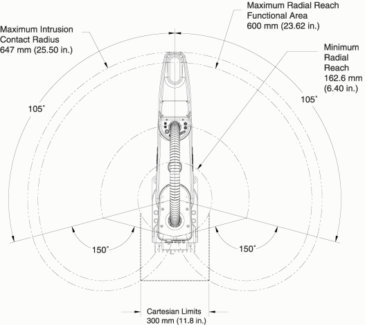
Fig. 46 Surface balayée par l’effecteur

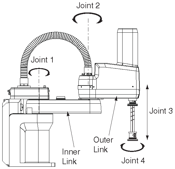
Fig. 47 Extrait de documentation : cinématique

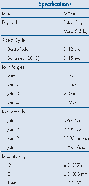
Fig. 48 Extrait de documentation : spécifications

Solution

Paramétrage du robot scara : cf TD 1