Correction du TD n°2 : MGI par la méthode de Paul, singularités

On étudie le robot 6 axes RX90 de marque Stäubli donné en Fig. 36} :

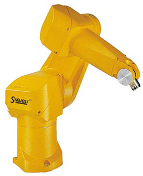
Fig. 36 Robot STAUBLI RX90

L’objectif du TD est de calculer l’ensemble des solutions au Modèle Géométrique Inverse (MGI) pour ce type de robot en utilisant la méthode de Paul. L’analyse de la résolution et des équations mises en jeu permet de déterminer les singularités du robot.

Analyse du paramétrage

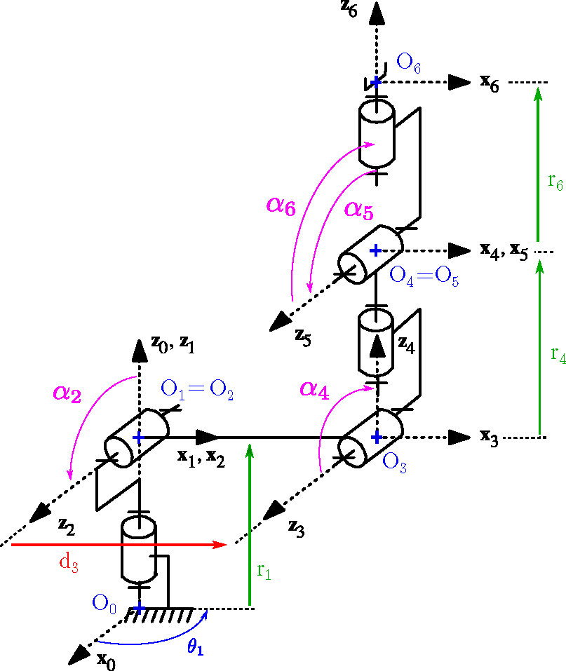
Le schéma cinématique du robot ainsi que le paramétrage selon la convention de Denavit et Hartenberg modifiée sont donnés en annexe.

Question 1.1 : Reporter sur le schéma cinématique les différents points caractéristiques, constantes géométriques, et paramètres articulaires.

Solution

Question 1.2 : Rappeler quelle est la particularité de cette structure permettant de découpler le problème de résolution du MGI en deux sous problèmes :

• le problème en position;

• le problème en orientation.

Solution

Le centre du poignet est l’intersection des axes de rotation concourants des 3 dernières liaisons pivots.

Dans cet exercice on cherche à établir le MGI. Par conséquent, on suppose la position et l’orientation de l’effecteur connues ! \(\mathcal{R}_6 = (O_6, \overrightarrow{x_6}, \overrightarrow{y_6}, \overrightarrow{z_6})\) connu ! Les paramètres du modèle de DHm sont aussi connus. Les seuls inconnus à déterminer dans cet exercice sont les paramètres articulaires.

Découpage du problème :

Connaissant \(\overrightarrow{z_6}\) et \(r_6 = cste\) on peut déterminer aisément la position du centre poignet (rotule équivalente) \(O_4 = O_5\). Les paramètres articulaires \(\theta_4\), \(\theta_5\) et \(\theta_6\) n’influent pas sur la position de \(O_4\) d’où : Le problème de position est fonction uniquement de \(\theta_1\), \(\theta_2\) et \(\theta_3\)

Une fois ce problème traité, \(\theta_1\), \(\theta_2\) et \(\theta_3\) sont connus. Le problème d’orientation nous permet d’obtenir les paramètres articulaires \(\theta_4\), \(\theta_5\) et \(\theta_6\).

Résolution du Modèle géométrique Inverse

Dans cette partie, il s’agit de mettre en oeuvre la méthode de résolution dite « de Paul » pour résoudre le MGI en deux temps.

Question 2.1 : Exprimer l’équation en position : expression de l’origine de \(O_4\) dans le référentiel de base \(\mathcal{R}_0\) en fonction des matrices de transformation homogènes mises en jeu. De quels paramètres articulaires dépend la position du point \(O_4\) ?

Solution

Expression de \(O_4\) dans le référentiel de base \(\mathcal{R}_{0}\) : \( ^0 P_4 = \mathbf{T}_{04}\ ^4P_4\). Dans la suite on notera : \(^0P_4 = (P_x, P_y, P_z)\).

\[\begin{split} \begin{equation*} \underbrace{\begin{pmatrix} P_x \\ P_y \\ P_z \\ 1 \end{pmatrix}}_{\substack{\text{connus car on} \\ \text{cherche le MGI}}} = \underbrace{\mathbf{T}_{01} \cdot \mathbf{T}_{12} \cdot \mathbf{T}_{23}}_{\substack{\theta_1, \, \theta_2, \, \theta_3, \\ \text{inconnues}}} \cdot \underbrace{ \mathbf{T}_{34} \cdot \begin{pmatrix} 0 \\ 0 \\ 0 \\ 1 \end{pmatrix} }_{\substack{\text{ne dépend} \\ \text{pas de } \theta_4}} \end{equation*} \end{split}\]

La position du point \(O_4\) dépend donc des seuls paramètres articulaires \(\theta_1\), \(\theta_2\) et \(\theta_3\).

Question 2.2 : Déterminer par la méthode de Paul l’ensemble des solutions articulaires obtenues par l’équation en position.

Solution

On aura besoin des matrices inverses \(\mathbf{T}_{10}\) et \(\mathbf{T}_{21}\)

Rappel de cours :

\[\begin{split} \begin{equation*} \text{si} \quad \mathbf{T}_{ij} = \begin{bmatrix} & & & \\ & \mathbf{R}_{ij} & & \mathbf{t}_{ij} \\ & & & \\ 0 & 0 & 0 & 1\\ \end{bmatrix} \quad \text{alors} \quad \mathbf{T}_{ji} = \mathbf{T}_{ij} ^{-1} = \begin{bmatrix} & & & \\ & \mathbf{R}_{ij} ^t & & -\mathbf{R}_{ij} ^t \mathbf{t}_{ij} \\ & & & \\ 0 & 0 & 0 & 1\\ \end{bmatrix} \end{equation*} \end{split}\]

\[\begin{split} \begin{align*} \mathbf{T}_{10}&= \begin{bmatrix} \text{C}\theta_1 & \text{S}\theta_1 & 0 & 0 \\ -\text{S}\theta_1 & \text{C}\theta_1 & 0 & 0 \\ 0 & 0 & 1 & -r_{1} \\ 0 & 0 & 0 & 1\\ \end{bmatrix} \\ \\ \mathbf{T}_{12}&= \begin{bmatrix} \text{C}\theta_2 & 0 & \text{S}\theta_2 & 0 \\ -\text{S}\theta_2 & 0 & \text{C}\theta_2 & 0 \\ 0 & -1 & 0 & 0 \\ 0 & 0 & 0 & 1\\ \end{bmatrix} \end{align*} \end{split}\]

Résolution en utilisant la méthode de Paul :

1 - Première étape :

\[\begin{split} \begin{align*} \begin{pmatrix} P_x \\ P_y \\ P_z \\ 1 \end{pmatrix} &= \mathbf{T}_{01} \cdot \mathbf{T}_{12} \cdot \mathbf{T}_{23} \cdot \mathbf{T}_{34} \cdot \begin{pmatrix} 0 \\ 0 \\ 0 \\ 1 \end{pmatrix} \\ \\ \mathbf{T}_{10} \cdot \begin{pmatrix} P_x \\ P_y \\ P_z \\ 1 \end{pmatrix} &= \mathbf{T}_{12} \cdot \mathbf{T}_{23} \cdot \begin{pmatrix} 0 \\ r4 \\ 0 \\ 1 \end{pmatrix} \\ \\ \begin{pmatrix} P_x \text{C}\theta_1 + P_y \text{S}\theta_1 \\ -P_x \text{S}\theta_1 + P_y \text{C}\theta_1 \\ P_z - r_1 \\ 1 \end{pmatrix} &= \mathbf{T}_{12} \cdot \begin{pmatrix} -r_4 \text{S}\theta_3 + d_3 \\ r4 \text{C}\theta_3 \\ 0 \\ 1 \end{pmatrix} \\ \\ \begin{pmatrix} P_x \text{C}\theta_1 + P_y \text{S}\theta_1 \\ -P_x \text{S}\theta_1 + P_y \text{C}\theta_1 \\ P_z - r_1 \\ 1 \end{pmatrix} &= \begin{pmatrix} (-r_4 \text{S}\theta_3 + d_3) \text{C}\theta_2 - r_4 \text{C}\theta_3 \text{S}\theta_2 \\ 0 \\ (-r_4 \text{S}\theta_3 + d_3) \text{S}\theta_2 + r_4 \text{C}\theta_3 \text{C}\theta_2 \\ 1 \end{pmatrix} \\ \\ \begin{pmatrix} P_x \text{C}\theta_1 + P_y \text{S}\theta_1 \\ -P_x \text{S}\theta_1 + P_y \text{C}\theta_1 \\ P_z - r_1 \\ 1 \end{pmatrix} &= \begin{pmatrix} -r_4 \text{S}(\theta_2 + \theta_3) + d_3 \text{C}\theta_2 \\ 0 \\ r_4 \text{C}(\theta_2 + \theta_3) + d_3 \text{S}\theta_2 \\ 1 \end{pmatrix} \end{align*} \end{split}\]

La seconde équation du système dépend uniquement de \(\theta_1\). Cette équation correspond à une équation de type 2 (cf. poly de cours) avec \(X = -P_x\), \(Y = P_y\) et \(Z = 0\) \

Cette équation admet deux solutions (cf. démonstration en annexes).

\[\begin{split} \begin{align*} \theta_{11} &= \text{atan2}(-P_y,-P_x)\\ \theta_{12} &= \theta_{11} + \pi \end{align*} \end{split}\]

2 - Deuxième étape :

La variable articulaire \(\theta_1\) est maintenant connue.

\[\begin{split} \begin{align*} \begin{pmatrix} P_x \\ P_y \\ P_z \\ 1 \end{pmatrix} &= \mathbf{T}_{01} \cdot \mathbf{T}_{12} \cdot \mathbf{T}_{23} \cdot \mathbf{T}_{34} \cdot \begin{pmatrix} 0 \\ 0 \\ 0 \\ 1 \end{pmatrix} \\ \\ \mathbf{T}_{21} \cdot \mathbf{T}_{10} \cdot \begin{pmatrix} P_x \\ P_y \\ P_z \\ 1 \end{pmatrix} &= \begin{pmatrix} -r_4 \text{S}\theta_3 + d_3 \\ r4 \text{C}\theta_3 \\ 0 \\ 1 \end{pmatrix} \\ \\ \begin{pmatrix} (P_x \text{C}\theta_1 + P_y \text{S}\theta_1)\text{C}\theta_2 + (P_z - r_1) \text{S}\theta_2 \\ -(P_x \text{C}\theta_1 + P_y \text{S}\theta_1)\text{S}\theta_2 + (P_z - r_1) \text{C}\theta_2 \\ P_x \text{S}\theta_1 - P_y \text{C}\theta_1 \\ 1 \end{pmatrix} &= \begin{pmatrix} -r_4 \text{S}\theta_3 + d_3 \\ r4 \text{C}\theta_3 \\ 0 \\ 1 \end{pmatrix} \end{align*} \end{split}\]

Les deux premières équations du système précédent permettent d’isoler \(\theta_2\). Pour cela, il suffit de déplacer \(d_3\) de l’autre côté de l’équation puis de faire la somme des deux équations au carré.

Pour simplifier les notations, on pose : \(c_1 = P_x \text{C}\theta_1 + P_y \text{S}\theta_1\) et \(c_2 = P_z - r_1\)

\[\begin{split} \begin{align*} ((1)-d_3)^2+(2)^2 \qquad \Rightarrow \qquad r_4^2 &= (c_1 \text{C}\theta_2 + c_2 \text{S}\theta_2 - d_3)^2 + (-c_1 \text{S}\theta_2 + c_2 \text{C}\theta_2)^2\\ \\ r_4^2 &= c_1^2 + c_2^2 - 2 d_3 c_2 \text{S}\theta_2 - 2 d_3 c_1 \text{C}\theta_2 + d_3^2\\ \\ r_4^2 - c_1^2 - c_2^2 - d_3^2 &= - 2 d_3 c_2 \text{S}\theta_2 - 2 d_3 c_1 \text{C}\theta_2 \end{align*} \end{split}\]

Cette équation correspond à une équation de type 2 (cf. poly de cours) avec \(X = - 2 d_3 c_2\), \(Y = - 2 d_3 c_1\) et \(Z = r_4^2 - c_1^2 - c_2^2 - d_3^2\)

Cette équation admet deux solutions (cf. démonstration en annexes).

\[\begin{split} \begin{align*} \theta_{21} &= \text{atan2}(\text{S}\theta_2 ,\text{C}\theta_2 ) \qquad \text{avec :} \qquad \varepsilon = +1 \\ \theta_{22} &= \text{atan2}(\text{S}\theta_2 ,\text{C}\theta_2 ) \qquad \text{avec :} \qquad \varepsilon = -1 \end{align*} \end{split}\]

\[\begin{split} \begin{equation*} \begin{cases} \text{C}\theta_2 = \dfrac{YZ - \varepsilon X \sqrt{X^2+Y^2-Z^2}}{X^2 + Y^2} \\ \text{S}\theta_2 = \dfrac{XZ + \varepsilon Y \sqrt{X^2+Y^2-Z^2}}{X^2 + Y^2} \\ \end{cases} \qquad \text{ et :} \qquad X^2 + Y^2 \geq Z^2 \end{equation*} \end{split}\]

3 - Troisième étape :

La variable articulaire \(\theta_2\) est maintenant connue. On peut en déduire \(\theta_3\). Pour cela on utilise les équations du système de l’étape 2.

\[\begin{split} \begin{align*} \begin{cases} \text{S}\theta_3 &= \dfrac{1}{r_4} \left[ -\text{C}\theta_2 (P_x \text{C}\theta_1 + P_y \text{s}\theta_1) -\text{S}\theta_2 (P_z -r_1) + d_3 \right] \\ \text{C}\theta_3 &= \dfrac{1}{r_4} \left[ -\text{S}\theta_2 (P_x \text{C}\theta_1 + P_y \text{s}\theta_1) +\text{C}\theta_2 (P_z -r_1) \right] \\ \end{cases} \\ \\ \text{d'ou :} \qquad \theta_3 = \text{atan2}( \text{S}\theta_3, \text{C}\theta_3) \end{align*} \end{split}\]

Question 2.3 : Exprimer l’équation en orientation : expression de la base orientant l’effecteur dans le référentiel de base \(\mathcal{B}_0\) en fonction des matrices de rotation (changement de bases) mises en jeu. Une fois le problème en position résolu, de quels paramètres articulaires dépend l’orientation de l’effecteur ?

Solution

Expression de la base effecteur dans la base 0

\[\begin{split} \begin{equation*} \underbrace{\begin{pmatrix} r_{11} & r_{12} & r_{13} \\ r_{21} & r_{22} & r_{23} \\ r_{31} & r_{32} & r_{33} \\ \end{pmatrix}}_{\substack{\text{matricce des cos} \\ \text{directeurs connus}}} = \mathbf{R}_{06}(\underbrace{\theta_1, \theta_2, \theta_3}_{\text{}Connus}, \theta_4, \theta_5, \theta_6) \end{equation*} \end{split}\]

On isole tous les termes connus en multipliant à gauche de chaque côté de l’équation par l’inverse de la matrice de rotation entre 0 et 3 : \(\mathbf{R}_{30}\).

\[\begin{split} \begin{equation*} \underbrace{\mathbf{R}_{30} \cdot \begin{pmatrix} r_{11} & r_{12} & r_{13} \\ r_{21} & r_{22} & r_{23} \\ r_{31} & r_{32} & r_{33} \\ \end{pmatrix}}_{\text{connus}} = \mathbf{R}_{36}(\theta_4, \theta_5, \theta_6) \end{equation*} \end{split}\]

Pour simplifier l’écriture, on renomme le terme de gauche :

\[\begin{split} \begin{equation*} \underbrace{\begin{pmatrix} F_x & G_x & H_x \\ F_y & G_y & H_y \\ F_z & G_z & H_z \\ \end{pmatrix}}_{\text{connus}} = \mathbf{R}_{36} \end{equation*} \end{split}\]

Maintenant que \(\theta_1\), \(\theta_2\), et \(\theta_3\) on cherche \(\theta_4\), \(\theta_5\), et \(\theta_6\) afin de répondre au problème en orientation.

Question 2.4 : Déterminer par la méthode de Paul l’ensemble des solutions articulaires obtenues par l’équation en orientation.

Solution

On procède de la même manière, mais sur l’équation en orientation.

\[\begin{split} \begin{align*} \mathbf{R}_{43} \cdot \begin{pmatrix} F_x & G_x & H_x \\ F_y & G_y & H_y \\ F_z & G_z & H_z \\ \end{pmatrix} &= \mathbf{R}_{46} \\ \\ \begin{pmatrix} \text{S}\theta_4 & 0 & -\text{S}\theta_4 \\ - \text{S}\theta_4 & 0 & -\text{C}\theta_4 \\ 0 & 1 & 0 \\ \end{pmatrix} \cdot \begin{pmatrix} F_x & G_x & H_x \\ F_y & G_y & H_y \\ F_z & G_z & H_z \\ \end{pmatrix} &= \begin{pmatrix} \text{C}\theta_5 \text{C}\theta_6 & - \text{C}\theta_5 \text{C}\theta_6 & - \text{S}\theta_5 \\ \text{S}\theta_6 & \text{C}\theta_6 & 0 \\ \text{S}\theta_5 \text{C}\theta_6 & - \text{S}\theta_5 \text{S}\theta_6 & \text{C}\theta_5 \\ \end{pmatrix} \end{align*} \end{split}\]

Cette équation matricielle nous donne 9 équations scalaires.

1 - L’équation \((2,3)\) permet de déterminer \(\theta_4\). effectivement il s’agit d’une équation de type 2 (cf. cours et démonstration).

\[ \begin{equation*} - H_x \text{S}\theta_4 - H_z \text{C}\theta_4 = 0 \end{equation*} \]

Cette équation admet deux solutions (cf. démonstration en annexes).

\[\begin{split} \begin{align*} \theta_{41} &= \text{atan2}(H_z,-H_x)\\ \theta_{42} &= \theta_{41} + \pi \end{align*} \end{split}\]

2 - Les équations \((1,3)\) et \((3,3)\) permettent de déterminer \(\theta_5\).

\[\begin{split} \begin{equation*} \begin{cases} - \text{S}\theta_5 &= H_x \text{C}\theta_4 - H_z \text{S}\theta_4\\ \text{C}\theta_5 &= H_y\\ \end{cases} \end{equation*} \end{split}\]

La solution est la suivante :

\[\begin{split} \begin{align*} \theta_{5} &= \text{atan2}(\text{S}\theta_5,\text{C}\theta_5)\\ \end{align*} \end{split}\]

3 - Les équations \((2,1)\) et \((2,2)\) permettent de déterminer \(\theta_6\).

\[\begin{split} \begin{equation*} \begin{cases} \text{S}\theta_6 &= - F_z \text{C}\theta_4 - F_x \text{S}\theta_4\\ \text{C}\theta_6 &= - G_z \text{C}\theta_4 - G_x \text{S}\theta_4\\ \end{cases} \end{equation*} \end{split}\]

La solution est la suivante :

\[\begin{split} \begin{equation*} \theta_{6} = \text{atan2}(\text{S}\theta_6,\text{C}\theta_6)\\ \end{equation*} \end{split}\]

Synthèse

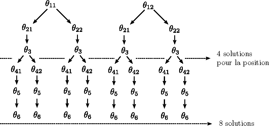
Question 3.1 : Faire le bilan sur le nombre de solutions articulaires correspondant à un positionnement du repère effecteur.

Solution

Synthèse du nombre de solutions articulaires pour une configuration de l’effecteur dans l’espace des tâches :

Question 3.2 : Importer le robot dans l’application « RoboDK », puis, sur quelques configurations, étudier les solutions (notamment leur nombre) au MGI.

Solution

Étant donné la course des paramètres articulaires, il existe dans certains cas, plus de 8 configurations articulaires permettant d’obtenir une position et une orientation de l’effecteur donnée. Si par contre on limite les courses articulaires à un seul et unique tour \((360 \deg)\), alors seules 8 configurations articulaires ou moins sont possibles (sauf au niveau des singularités).

Question 3.3 : À partir des équations obtenues en partie 2, déterminer et illustrer les singularités géométriques de ce robot.

Solution

Singularité : Une infinité de solutions dans l’espace articulaire donne la même configuration dans l’espace des tâches.

• Pour le calcul de \(\theta_1\) : si \(P_x = P_y = 0\) cela implique que \(\theta_1\) est indéterminé (singularité au niveau de l’épaule)

• Pour le calcul de \(\theta_4\) : si \(H_x = H_z = 0\) cela implique que \(\theta_4\) est indéterminé (singularité au niveau du poignet)

• Singularité au niveau du coude : déplacement possible uniquement dans une direction.

Annexes

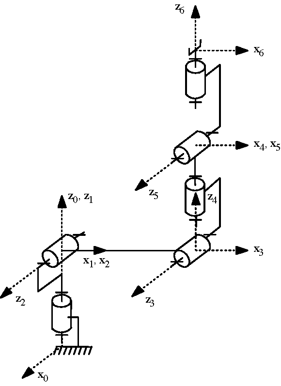
Fig. 37 Schéma cinématique

	\(d_i\)	\(\alpha_i\)	\(r_i\)	\(\theta_i\)
\(\mathbf{T}_{01}\)	0	0	\(r_1\)	\(\theta_1\)
\(\mathbf{T}_{12}\)	0	\(90^{\circ}\)	0	\(\theta_2\)
\(\mathbf{T}_{23}\)	\(d_3\)	0	0	\(\theta_3\)
\(\mathbf{T}_{34}\)	0	\(-90^{\circ}\)	\(r_4\)	\(\theta_4\)
\(\mathbf{T}_{45}\)	0	\(90^{\circ}\)	0	\(\theta_5\)
\(\mathbf{T}_{56}\)	0	\(-90^{\circ}\)	\(r_6\)	\(\theta_6\)

Matrices homogènes élémentaires de transformations entre repères :

\[\begin{split} \begin{align*} \mathbf{T}_{01}&= \begin{bmatrix} \text{C}\theta_1 & -\text{S}\theta_1 & 0 & 0 \\ \text{S}\theta_1 & \text{C}\theta_1 & 0 & 0 \\ 0 & 0 & 1 & r_{1} \\ 0 & 0 & 0 & 1\\ \end{bmatrix} \\ \\ \mathbf{T}_{12}&= \begin{bmatrix} \text{C}\theta_2 & -\text{S}\theta_2 & 0 & 0 \\ 0 & 0 & -1 & 0 \\ \text{S}\theta_2 & \text{C}\theta_2 & 0 & 0 \\ 0 & 0 & 0 & 1\\ \end{bmatrix} \\ \\ \mathbf{T}_{23}&= \begin{bmatrix} \text{C}\theta_3 & -\text{S}\theta_3 & 0 & d_3 \\ \text{S}\theta_3 & \text{C}\theta_3 & 0 & 0 \\ 0 & 0 & 1 & 0 \\ 0 & 0 & 0 & 1\\ \end{bmatrix} \\ \\ \mathbf{T}_{34}&= \begin{bmatrix} \text{C}\theta_4 & -\text{S}\theta_4 & 0 & 0 \\ 0 & 0 & 1 & r_4 \\ -\text{S}\theta_4 & -\text{C}\theta_4 & 0 & 0 \\ 0 & 0 & 0 & 1\\ \end{bmatrix} \\ \\ \mathbf{T}_{45}&= \begin{bmatrix} \text{C}\theta_5 & -\text{S}\theta_5 & 0 & 0 \\ 0 & 0 & -1 & 0 \\ \text{S}\theta_5 & \text{C}\theta_5 & 0 & 0 \\ 0 & 0 & 0 & 1\\ \end{bmatrix} \\ \\ \mathbf{T}_{56}&= \begin{bmatrix} \text{C}\theta_6 & -\text{S}\theta_6 & 0 & 0 \\ 0 & 0 & 1 & r_6 \\ -\text{S}\theta_6 & -\text{C}\theta_6 & 0 & 0 \\ 0 & 0 & 0 & 1\\ \end{bmatrix} \end{align*} \end{split}\]

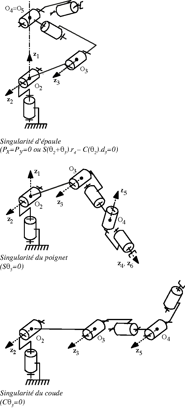
Fig. 38 Positions singulières

Solution

Solutions de l’équation de type 2 :

\[ \begin{equation*} X \text{S}\theta_i + Y \text{C}\theta_i = Z \end{equation*} \]

Solution :

\[\begin{split} \begin{align*} \theta_i = \begin{cases} \text{atan2}(\pm \sqrt{1 - \text{C}^2\theta_i},\, \text{C}\theta_i) \quad & \text{si} \quad X = 0 \text{ et } Y \ne 0 \\ \text{atan2}(\text{S}\theta_i, \, \pm \sqrt{1 - \text{S}^2\theta_i}) \quad & \text{si} \quad X \ne 0 \text{ et } Y = 0 \\ \begin{cases} \theta_{i1} = \text{atan2}(-Y,X) \\ \theta_{i2} = \theta_{i1} + 180\deg \end{cases} \quad & \text{si} \quad X \ne 0 \text{ et } Y \ne 0 \text{ et } Z = 0 \\ \text{atan2}(\text{S}\theta_i, \, \text{C}\theta_i) \quad & \text{si} \quad X \ne 0 \text{ et } Y \ne 0 \text{ et } Z \ne 0 \text{ et } X^2+Y^2 \geq Z^2 \\ \text{configuration singulière} \quad & \text{si} \quad X \ne 0 \text{ et } Y \ne 0 \\ \end{cases} \end{align*} \end{split}\]

Dans le cas où \(X \ne 0\) et \(Y \ne 0\) et \(Z \ne 0\), l’équation est résolue en élevant l’expression au carré : en remplaçant les termes en sinus par les fonctions équivalentes en cosinus, on aboutit à une équation du second degré à résoudre donnant la valeur du cosinus. Un raisonnement analogue est mené pour déterminer le terme en sinus :

\[\begin{split} \begin{equation*} \begin{cases} \text{C}\theta_2 = \dfrac{YZ - \varepsilon X \sqrt{X^2+Y^2-Z^2}}{X^2 + Y^2} \\ \text{S}\theta_2 = \dfrac{XZ + \varepsilon Y \sqrt{X^2+Y^2-Z^2}}{X^2 + Y^2} \\ \end{cases} \qquad \text{avec} \qquad \varepsilon = \pm 1 \end{equation*} \end{split}\]

Dans ce cas, la résolution de l’équation donne deux solutions, correspondant aux valeurs de \(\varepsilon\).